§112 (8 Ed §101)
Definition. A conformal map f is a map f : z \mapsto w where f is analytic and f'(z_0) \ne 0. Then locally (near z_0), f preserves angles, orientation, and shape.
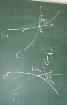
In the image below, \Gamma_1 and \Gamma_2 are the images of C_1 and C_2 under f. The angles between them are \alpha and \beta. They intersect at z_0 and f(z_0), respectively. That is, \Gamma_1 = f(C_1) and \Gamma_2=f(C_2). Conformality tells us that \alpha = \beta.
If orientation (i.e. sense, direction) is not necessarily preserved but the angle’s magnitude is, the map is called isogonal.
If instead we had an analytic function with f'(z_0)=0, then z_0 is a critical point of f. This means the angle is not preserved around z_0. However, the angle will be multiplied by m where m is the smallest integer such that f^{(m)}(z_0) \ne 0.
§113 (8 Ed §103)
Conformality means the map is locally 1-to-1 and onto. That is, f has a local inverse. This follows from MATH2400/1’s inverse function theorem. Specifically, it is locally invertible if \det J_f \ne 0. In this case, \begin{aligned} \det J_f = \begin{vmatrix}u_x & u_y \\ v_x & v_y\end{vmatrix} = u_x v_y - u_y v_x = u_x^2 + v_x^2 = |u_x + iv_x|^2 = |f'|^2 \ne 0 \end{aligned} due to f'(z_0) \ne 0 and analyticity of f.
We look for a function U : \Omega \to \mathbb R such that \Delta U = 0 \quad\text{(or alternatively, }\nabla^2U=0\text{)}.
Here, \Delta or \nabla^2 is the Laplacian/Laplace operator defined as \Delta U = U_{xx} + U_{yy} or more generally in \mathbb R^n, \Delta = \sum_{j=1}^n U_{jj}. This is used to model many physical situations in “steady state”.
Take a region \Omega \subset \mathbb R^2 or \mathbb R^3. Let \Lambda be a “sufficiently smooth subdomain of \Omega”. Some intuition is that an arbitrary point \mathbf x on the \partial \Lambda has an external normal, denoted \boldsymbol{\nu}(\mathbf x) with unit normal \boldsymbol{\nu}'(\mathbf x).
U is the density of something “in equilibrium”, and \mathbf F is the flux density of U in \Omega “in equilibrium”.
This means that along the boundary of \Lambda, \int_{\partial \Lambda} \mathbf F \cdot \boldsymbol{\nu}'\,dS = 0, where dS is the surface measure on \partial \Lambda (i.e. one dimension lower). This means the net in-flow and out-flow are equal. In terms of fluids, this means there are no sources and sinks.
We apply Gauss divergence theorem with the above integral which tells us that \int_{\partial \Lambda} \mathbf F \cdot \boldsymbol{\nu}'\,dS=\int_\Lambda \operatorname{div}\mathbf F\,d\mathbf x = 0 where d\mathbf x = dx\,dy in 2D, etc. Since \Lambda is essentially arbitrary, there holds \operatorname{div}\mathbf F = 0 in \Omega. That is, \sum_{j=1}^n \partial_j F_j = 0 in \Omega.
In many physical situations, \mathbf F = c \nabla U with c usually negative (corresponding to repelling forces). This means that \begin{aligned} \operatorname{div}\mathbf F &= c\operatorname{div}\nabla U = 0 \implies \operatorname{div} \nabla U = \Delta U = 0. \end{aligned}